KaKs Vignette
Kristian K Ullrich
2023-12-22
Source:vignettes/V02KaKsVignette.Rmd
V02KaKsVignette.RmdKa/Ks Vignette
- includes Arabidopsis thalina and Arabidopsis lyrata CRBHit pair calculation
- includes Homo sapiens and Pan troglodytes CRBHit pair calculation
- inlcudes Longest Isoform selection
- includes Gene/Isoform chromosomal position extraction
- includes Tandem Duplicate Assignment
- includes Synteny Assignment
- includes Ka/Ks colored Dot-Plot
Table of Contents
- Conditional Reciprocal Best Hit pairs (CRBH pairs)
- Ka/Ks Calculation
- Ka/Ks Filtering and Visualisation
- Homo sapiens vs. Pan troglodytes example
- References
This vignette is supposed to explain in more detail Ka/Ks calculation and it’s downstream filtering and visualization. The Ka/Ks ratio was originally developed for the analysis of genetic sequences from divergent species (Kimura (1977), Yang and Nielson (2000)). In short, the Ka/Ks ratio quantifies the mode and strength of selection by comparing synonymous substitution rates (Ks) (assumed to be evolutionary neutral) with nonsynonymous rates (Ka), which are exposed to selection as they change the amino acid composition of a protein (Mugal et al (2014)).
CRBHits is a reimplementation of the Conditional Reciprocal Best Hit (CRBH) algorithm crb-blast in R. The CRBHit pairs can be directly used to calculate Ka/Ks ratios and to filter for tandem duplicates or syntenic groups.
See the R package page for a detailed description of the install process and its dependencies https://mpievolbio-it.pages.gwdg.de/crbhits/ or have a look at the CRBHits Basic Vignette.
Note:
In this Vignette the lastpath is defined as
vignette.paths[1], the kakscalcpath as
vignette.paths[2] and the dagchainerpath as
vignette.paths[3] to be able to build the Vignette.
However, once you have compiled last-1521, KaKs_Calculator2.0 and
DAGchainer with the functions make_last(),
make_KaKs_Calculator2() and make_dagchainer()
you won’t need to specify the paths anymore. Please remove them if you
would like to repeat the examples.
## load vignette specific libraries
library(CRBHits)
suppressPackageStartupMessages(library(Biostrings))
suppressPackageStartupMessages(library(dplyr))
suppressPackageStartupMessages(library(ggplot2))
suppressPackageStartupMessages(library(gridExtra))
suppressPackageStartupMessages(library(curl))
## compile LAST, KaKs_Calculator2.0 and DAGchainer for the vignette
vignette.paths <- make_vignette()
1. Conditional reciprocal best hit pairs
The CRBH algorithm builds upon the classical reciprocal best hit (RBH) approach to find orthologous sequences between two sets of sequences by defining an expect-value cutoff per alignment length. Further, this cutoff is used to retain secondary hits as additional bona-fide homologues.
See the R package page and the CRBHits Basic Vignette for a more detailed description of the CRBH algorithm.
1.1. Download Coding sequences (CDS) from NCBI and ENSEMBL
To calculate CRBHit pairs between two species, one can directly use an URL to access the coding sequences and calculate the CRBH pairs matrix.
Two examples are given in this vignette.
The first example compares the coding sequences from Arabidopsis thaliana and Arabidopsis lyrata. The input sequences are from the FTP server from NCBI Genomes.
The second example compares the CDS from Homo sapiens and Pan troglodytes (see Homo sapiens vs. Pan troglodytes example).
As an alternative the EnsemblPlants release-52 can used.
## set URLs for Arabidopis thaliana and Arabidopsis lyrata from NCBI Genomes

## set NCBI URL
NCBI <- "https://ftp.ncbi.nlm.nih.gov/genomes/all/"

## set Arabidopsis thaliana CDS URL
ARATHA.cds.url <- paste0(NCBI, "GCF/000/001/735/GCF_000001735.4_TAIR10.1/",
    "GCF_000001735.4_TAIR10.1_cds_from_genomic.fna.gz")

## set Arabidopsis lyrata CDS URL
ARALYR.cds.url <- paste0(NCBI, "GCF/000/004/255/GCF_000004255.2_v.1.0/",
    "GCF_000004255.2_v.1.0_cds_from_genomic.fna.gz")

## get Arabidopsis thaliana CDS
ARATHA.cds <- Biostrings::readDNAStringSet(ARATHA.cds.url)
## get Arabidopsis lyrata CDS
ARALYR.cds <- Biostrings::readDNAStringSet(ARALYR.cds.url)
1.2. Get Longest Isoform from NCBI or ENSEMBL Input
Prior CRBHit pairs calculation, the longest isoforms can be selected, if the data was downloaded from NCBI or Ensembl.
Note: This is an important step. If e.g. isoforms are used, the Ka/Ks calculations might show biased values inspecting mean or median Ka/Ks values grouped per query sequence.
1.2.1 isoform2longest()
## get longest isoform from sequence IDs
ARATHA.cds.longest <- isoform2longest(ARATHA.cds, "NCBI")
ARALYR.cds.longest <- isoform2longest(ARALYR.cds, "NCBI")

## get help
#?isoform2longest
1.2.2 gtf2longest()
Note: Sometimes the sequence IDs do not have the
necessary information to extract the longest isoforms. If this might be
the case, please use the dedicated functions gtf2longest()
or gff2longest() to get the gene positions and the longest
isoforms.
## set NCBI URL
NCBI <- "https://ftp.ncbi.nlm.nih.gov/genomes/all/"

ARATHA.NCBI.cds.url <- paste0(NCBI, "GCF/000/001/735/GCF_000001735.4_TAIR10.1/",
    "GCF_000001735.4_TAIR10.1_cds_from_genomic.fna.gz")
ARALYR.NCBI.cds.url <- paste0(NCBI, "GCF/000/004/255/GCF_000004255.2_v.1.0/",
    "GCF_000004255.2_v.1.0_cds_from_genomic.fna.gz")
ARATHA.NCBI.cds <- Biostrings::readDNAStringSet(ARATHA.NCBI.cds.url)
ARALYR.NCBI.cds <- Biostrings::readDNAStringSet(ARALYR.NCBI.cds.url)

## get longest isoform from GTF file - NCBI

## set Arabidopsis thaliana GTF URL
ARATHA.NCBI.gtf.url <- paste0(NCBI, "GCF/000/001/735/GCF_000001735.4_TAIR10.1/",
    "GCF_000001735.4_TAIR10.1_genomic.gtf.gz")
ARALYR.NCBI.gtf.url <- paste0(NCBI, "GCF/000/004/255/GCF_000004255.2_v.1.0/",
    "GCF_000004255.2_v.1.0_genomic.gtf.gz")

## get longest isoform from GTF file
ARATHA.NCBI.gtf.longest <- gtf2longest(
    gtffile=ARATHA.NCBI.gtf.url,
    cds=ARATHA.NCBI.cds,
    removeNonCoding=TRUE,
    source="NCBI")
ARALYR.NCBI.gtf.longest <- gtf2longest(
    gtffile=ARALYR.NCBI.gtf.url,
    cds=ARALYR.NCBI.cds,
    removeNonCoding=TRUE,
    source="NCBI")

ARATHA.NCBI.gtf.cds.longest <- ARATHA.NCBI.gtf.longest$cds
ARALYR.NCBI.gtf.cds.longest <- ARALYR.NCBI.gtf.longest$cds

ARATHA.NCBI.gtf.cds.genepos <- ARATHA.NCBI.gtf.longest$genepos
ARALYR.NCBI.gtf.cds.genepos <- ARALYR.NCBI.gtf.longest$genepos

## get help
#?gtf2longest
## set ENSEMBL URL
ENSEMBL <- "http://ftp.ensemblgenomes.org/pub/plants/release-52/"
ARATHA.ENSEMBL.cds.url <- paste0(ENSEMBL,
"fasta/arabidopsis_thaliana/cds/",
"Arabidopsis_thaliana.TAIR10.cds.all.fa.gz")
ARALYR.ENSEMBL.cds.url <- paste0(ENSEMBL,
"fasta/arabidopsis_lyrata/cds/",
"Arabidopsis_lyrata.v.1.0.cds.all.fa.gz")
ARATHA.ENSEMBL.cds <- Biostrings::readDNAStringSet(ARATHA.ENSEMBL.cds.url)
ARALYR.ENSEMBL.cds <- Biostrings::readDNAStringSet(ARALYR.ENSEMBL.cds.url)
## get longest isoform from GTF file - ENSEMBL
## set Arabidopsis thaliana GTF URL
ARATHA.ENSEMBL.gtf.url <- paste0(ENSEMBL, "gtf/arabidopsis_thaliana/",
"Arabidopsis_thaliana.TAIR10.52.gtf.gz")
ARALYR.ENSEMBL.gtf.url <- paste0(ENSEMBL, "gtf/arabidopsis_lyrata/",
"Arabidopsis_lyrata.v.1.0.52.gtf.gz")
## get longest isoform from GTF file
ARATHA.ENSEMBL.gtf.longest <- gtf2longest(
gtffile=ARATHA.ENSEMBL.gtf.url,
cds=ARATHA.ENSEMBL.cds,
removeNonCoding=TRUE,
source="ENSEMBL")
ARALYR.ENSEMBL.gtf.longest <- gtf2longest(
gtffile=ARALYR.ENSEMBL.gtf.url,
cds=ARALYR.ENSEMBL.cds,
removeNonCoding=TRUE,
source="ENSEMBL")
ARATHA.ENSEMBL.gtf.cds.longest <- ARATHA.ENSEMBL.gtf.longest$cds
ARALYR.ENSEMBL.gtf.cds.longest <- ARALYR.ENSEMBL.gtf.longest$cds
ARATHA.ENSEMBL.gtf.cds.genepos <- ARATHA.ENSEMBL.gtf.longest$genepos
ARALYR.ENSEMBL.gtf.cds.genepos <- ARALYR.ENSEMBL.gtf.longest$genepos
## get help
#?gtf2longest1.2.3 gff2longest()
## set NCBI URL
NCBI <- "https://ftp.ncbi.nlm.nih.gov/genomes/all/"

## get longest isoform from GFF3 file - NCBI

## set Arabidopsis thaliana GFF3 URL
ARATHA.NCBI.gff3.url <- paste0(NCBI, "GCF/000/001/735/GCF_000001735.4_TAIR10.1/",
    "GCF_000001735.4_TAIR10.1_genomic.gff.gz")
ARALYR.NCBI.gff3.url <- paste0(NCBI, "GCF/000/004/255/GCF_000004255.2_v.1.0/",
    "GCF_000004255.2_v.1.0_genomic.gff.gz")

## get longest isoform from GFF3 file
ARATHA.NCBI.gff3.longest <- gff2longest(
    gff3file=ARATHA.NCBI.gff3.url,
    cds=ARATHA.NCBI.cds,
    removeNonCoding=TRUE,
    source="NCBI")
ARALYR.NCBI.gff3.longest <- gff2longest(
    gff3file=ARALYR.NCBI.gff3.url,
    cds=ARALYR.NCBI.cds,
    removeNonCoding=TRUE,
    source="NCBI")

ARATHA.NCBI.gff3.cds.longest <- ARATHA.NCBI.gff3.longest$cds
ARALYR.NCBI.gff3.cds.longest <- ARALYR.NCBI.gff3.longest$cds

ARATHA.NCBI.gff3.cds.genepos <- ARATHA.NCBI.gff3.longest$genepos
ARALYR.NCBI.gff3.cds.genepos <- ARALYR.NCBI.gff3.longest$genepos

## get help
#?gff2longest
## set ENSEMBL URL
ENSEMBL <- "http://ftp.ensemblgenomes.org/pub/plants/release-52/"
## get longest isoform from GFF3 file - ENSEMBL
## set Arabidopsis thaliana GFF3 URL
ARATHA.ENSEMBL.gff3.url <- paste0(ENSEMBL, "gff3/arabidopsis_thaliana/",
"Arabidopsis_thaliana.TAIR10.52.gff3.gz")
ARALYR.ENSEMBL.gff3.url <- paste0(ENSEMBL, "gff3/arabidopsis_lyrata/",
"Arabidopsis_lyrata.v.1.0.52.gff3.gz")
ARATHA.ENSEMBL.gff3.file <- tempfile()
download.file(ARATHA.ENSEMBL.gff3.url, ARATHA.ENSEMBL.gff3.file, quiet=FALSE)
ARALYR.ENSEMBL.gff3.file <- tempfile()
download.file(ARALYR.ENSEMBL.gff3.url, ARALYR.ENSEMBL.gff3.file, quiet=FALSE)
## get longest isoform from GFF3 file
ARATHA.ENSEMBL.gff3.longest <- gff2longest(
gff3file=ARATHA.ENSEMBL.gff3.file,
cds=ARATHA.ENSEMBL.cds,
removeNonCoding=TRUE,
source="ENSEMBL")
ARALYR.ENSEMBL.gff3.longest <- gff2longest(
gff3file=ARALYR.ENSEMBL.gff3.file,
cds=ARALYR.ENSEMBL.cds,
removeNonCoding=TRUE,
source="ENSEMBL")
ARATHA.ENSEMBL.gff3.cds.longest <- ARATHA.ENSEMBL.gff3.longest$cds
ARALYR.ENSEMBL.gff3.cds.longest <- ARALYR.ENSEMBL.gff3.longest$cds
ARATHA.ENSEMBL.gff3.cds.genepos <- ARATHA.ENSEMBL.gff3.longest$genepos
ARALYR.ENSEMBL.gff3.cds.genepos <- ARALYR.ENSEMBL.gff3.longest$genepos
## get help
#?gff2longest1.3. Calculate/Filter CRBHit pairs
The blast-like software LAST is used to compare the translated CDS against each other and output a blast-like output table including the query and target length.
The hit pairs are filtered prior fitting for a query coverage of 50% and the twilight zone of protein sequence alignments (Rost B. (1999)).
The CRBhit pairs can be calculated directly from the URLs with the
function cdsfile2rbh() using multiple threads including
longest isoform selection.
For a detailed description of the cdsfile2rbh() function
and the cds2rbh() function with its individual filtering
steps prior CRBH algorithm fitting see the CRBHits
Basic Vignette.
## calculate CRBHit pairs for A. thaliana and A. lyrata using 2 threads

## input from CDS obtained from NCBI
## longest isoform selection
## query coverage >= 50%
## rost199 filter
ARATHA_ARALYR_crbh <- cds2rbh(
    cds1=ARATHA.cds,
    cds2=ARALYR.cds,
    qcov=0.5,
    rost1999=TRUE,
    longest.isoform=TRUE,
    isoform.source="NCBI",
    threads=2,
    plotCurve=TRUE,
    lastpath=vignette.paths[1])
attributes(ARATHA_ARALYR_crbh)$selfblast

## get help
#?cds2rbh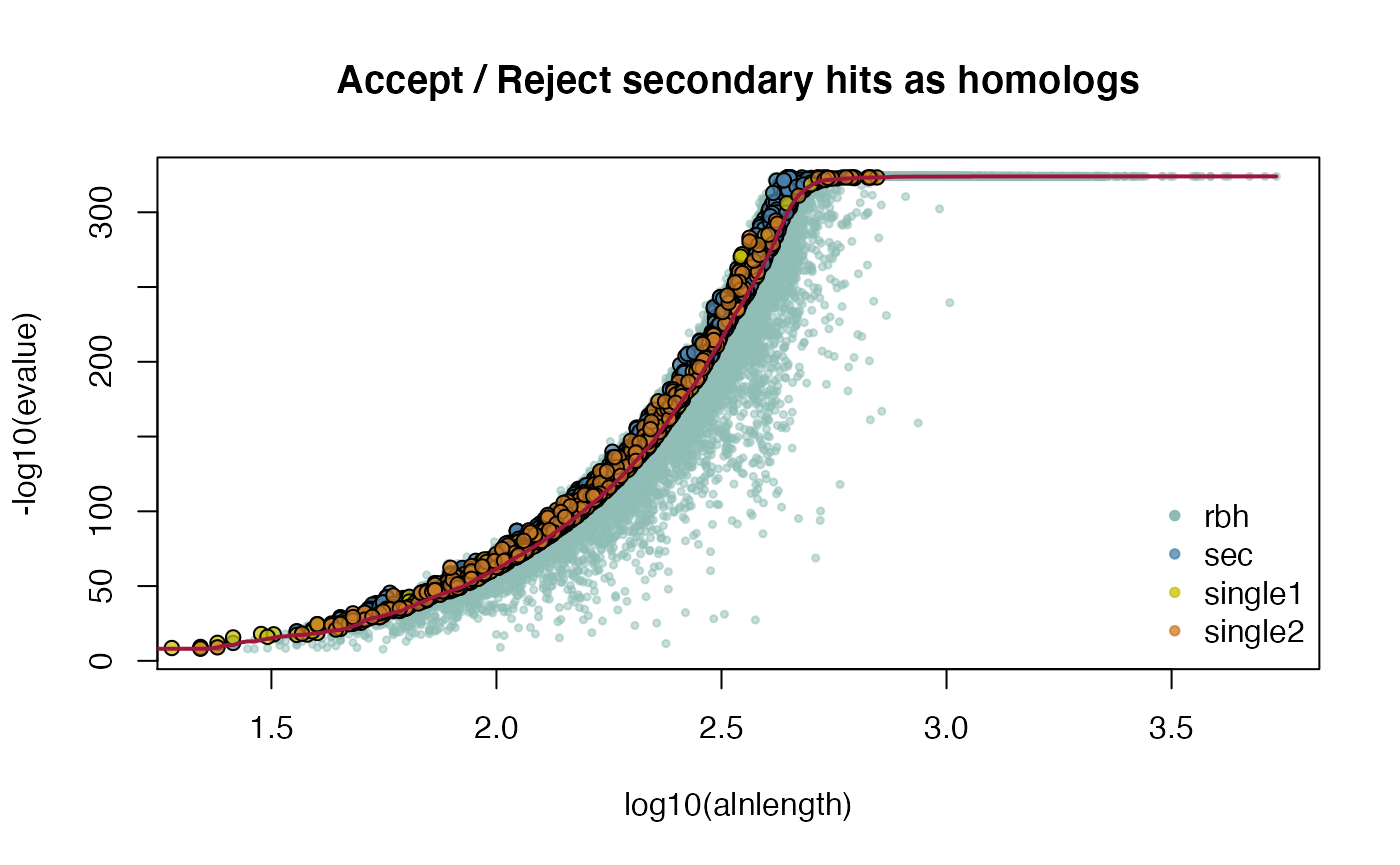
1.4. Extract Gene/Isoform chromosomal position
To be able to filter for Tandem Duplicates and to plot a
dotplot, one needs to have annotated gene positions per
chromosome/contig. With the cds2genepos() function it is
possible to directly access this information if the data was obtained
from NCBI or Ensembl.
Chromosomal gene positions might overlap and if one has not filtered to use the longest or primary isoform there will be positions overlap for CDS. To overcome this issue it is recommended to first reduce the CDS Input to the longest isoform (see Get Longest Isoform from NCBI or ENSEMBL Input).
Note: It is also possible to obtain and define chromosomal gene positions from other sources, like parsing a GTF/GFF file and supply a manual curated genepos matrix. In the same way this process might be used to select the longest/primary isoform from CDS Input sources other than NCBI or Ensembl. This special case is handled here:
1.4.1. Get gene position from NCBI or ENSEMBL Input
If the CDS Input was obtained from NCBI or ENSEMBL, the gene position
can be directly extracted from the DNAStringSet as
follows.
Note: Sometimes the sequence IDs do not have the
necessary information to extract the longest isoforms. If this might be
the case, please use the dedicated functions gtf2longest()
or gff2longest() to get the gene positions and the longest
isoforms.
## get gene position idx from NCBI CDS

## extract gene position from CDS directly from sequence IDs
ARATHA.cds.genepos <- cds2genepos(
    cds=ARATHA.cds,
    source="NCBI")
## extract gene position from longest isoform CDS
ARATHA.cds.longest.genepos <- cds2genepos(
    cds=ARATHA.cds.longest,
    source="NCBI")
## show first entries
head(ARATHA.cds.genepos)
head(ARATHA.cds.longest.genepos)
## get number of gene isoforms with same index
table(table(ARATHA.cds.genepos$gene.idx))
table(table(ARATHA.cds.longest.genepos$gene.idx))

##get help
#?cds2genepos
1.4.2. Use GTF/GFF3 file to obtain gene position
As noted above, it is also possible to obtain gene position and corresponding the longest isoforms per gene annotated in a GTF/GFF3 file.
see GTF/GFF3 format
Note: In some cases the IDs provided in the CDS and the GTF/GFF3 file differ, which make it more complicated to directly link gene position and CDS.
Here, as an example, the GTF file for the species Arabidopsis thaliana is obtained from the FTP server from Ensembl Plants.
Note: The GTF and GFF3 files can be very large and it might take some time until this data is loaded into memory.
see gtf2longest() in section 1.2.2 and
gff2longest() in section 1.2.3
Note: These manual steps (see below) are now
deprecated, please use the dedicated functions
gtf2longest() or gff2longest().
## deprecated, please use gtf2longest() or gff2longest() function
## get gene position idx from GTF/GFF3

## set NCBI URL
ensemblPlants <- "ftp://ftp.ensemblgenomes.org/pub/plants/release-48/"
## set Arabidopsis thaliana GFF3 URL
ARATHA.GFF.url <- paste0(ensemblPlants, "gff3/arabidopsis_thaliana/",
    "Arabidopsis_thaliana.TAIR10.48.gff3.gz")
## downlaod and gunzip file
ARATHA.GFF.file <- tempfile()
ARATHA.GFF.file.gz <- paste0(ARATHA.GFF.file, ".gz")
download.file(ARATHA.GFF.url, ARATHA.GFF.file.gz, quiet=FALSE)
system2(command="gunzip", args=c("-f", ARATHA.GFF.file.gz))
## read ARATHA.GFF.file
ARATHA.gff <- read.table(ARATHA.GFF.file, sep="\t",
    quote="", header=FALSE)
colnames(ARATHA.gff) <- c("seqname", "source", "feature", "start", "end",
    "score", "strand", "frame", "attribute")

## extract gene
ARATHA.gff.gene <- ARATHA.gff %>% dplyr::filter(feature=="gene")
## get gene ID
ARATHA.gff.gene.id <- gsub("ID\\=", "",
    stringr::word(ARATHA.gff.gene$attribute, 1, sep=";"))
## extract mRNA
ARATHA.gff.mRNA <- ARATHA.gff %>% dplyr::filter(feature=="mRNA")
## get mRNA ID
ARATHA.gff.mRNA.id <- gsub("ID\\=", "",
    stringr::word(ARATHA.gff.mRNA$attribute, 1, sep=";"))
## get mRNA based gene ID
ARATHA.gff.mRNA.parent.id <- gsub("Parent\\=", "",
    stringr::word(ARATHA.gff.mRNA$attribute, 2, sep=";"))
## add mRNA ID and mRNA based gene ID
ARATHA.gff.mRNA <- ARATHA.gff.mRNA %>%
    dplyr::mutate(gene.id=ARATHA.gff.mRNA.parent.id,
    mRNA.id=ARATHA.gff.mRNA.id)
## extract CDS
ARATHA.gff.CDS <- ARATHA.gff %>% dplyr::filter(feature=="CDS")
## get CDS based mRNA ID
ARATHA.gff.CDS.parent.id <- gsub("Parent\\=", "",
    stringr::word(ARATHA.gff.CDS$attribute, 2, sep=";"))
## add CDS based mRNA ID
ARATHA.gff.CDS <- ARATHA.gff.CDS %>%
    dplyr::mutate(mRNA.id=ARATHA.gff.CDS.parent.id)
## get width per mRNA isoform
ARATHA.gff.mRNA.len <- ARATHA.gff.CDS %>% dplyr::group_by(mRNA.id) %>%
    dplyr::summarise(mRNA.id=unique(mRNA.id),
    len=sum(end-start+1))
## add mRNA isoform width
ARATHA.gff.mRNA <- ARATHA.gff.mRNA %>%
    dplyr::mutate(mRNA.len=
    ARATHA.gff.mRNA.len$len[
    match(ARATHA.gff.mRNA$mRNA.id,
    ARATHA.gff.mRNA.len$mRNA.id)])
## retain only longest mRNA isoform
ARATHA.gff.mRNA.longest <- ARATHA.gff.mRNA %>%
    dplyr::arrange(seqname, desc(mRNA.len), mRNA.id, gene.id, start) %>%
    dplyr::distinct(gene.id, .keep_all=TRUE) %>%
    dplyr::mutate(gene.mid=start + (end-start)/2)
## add gene idx
ARATHA.gff.mRNA.longest <- ARATHA.gff.mRNA.longest %>%
  dplyr::mutate(gene.idx=seq(from=1, to=dim(ARATHA.gff.mRNA.longest)[1]))
## create gene position matrix to be used for downstream analysis
ARATHA.gff.genepos <- ARATHA.gff.mRNA.longest %>%
    dplyr::select(
    gene.seq.id=mRNA.id,
    gene.chr=seqname,
    gene.start=start,
    gene.end=end,
    gene.mid=gene.mid,
    gene.strand=strand,
    gene.idx=gene.idx)
## set attribute
attr(ARATHA.gff.genepos, "CRBHits.class") <- "genepos"
## show first entries of generated gene position
head(ARATHA.gff.genepos)
1.5 Assign Tandem Duplicates
Tandem duplicated genes (gene family members that are tightly clustered on a chromosome) are common in plant genomes and can show different Ka/Ks distribution than non tandem duplicates or other segmental duplicated genes (Rizzon et al., 2006).
In order to account for this, it is possible to classify these tandem
duplicates with the tandemdups() function.
Note: To be able to classify tandem duplicated genes within one genome, one needs to calculate selfblast based CRBHit pairs and provide gene position information for the same input data.
The following example shows how one can:
- get selfblast CRBHit pairs
- get gene positions
- assign tandem duplicates
## example to assign tandem duplicates given selfblast CRBHit pairs and gene position

## get selfblast CRBHit pairs for A. thaliana
ARATHA_selfblast_crbh <- cds2rbh(
    cds1=ARATHA.cds,
    cds2=ARATHA.cds,
    qcov=0.5,
    rost1999=TRUE,
    longest.isoform=TRUE,
    isoform.source="NCBI",
    threads=2,
    plotCurve=TRUE,
    lastpath=vignette.paths[1])
attributes(ARATHA_selfblast_crbh)$selfblast
## get selfblast CRBHit pairs for A. lyrata
ARALYR_selfblast_crbh <- cds2rbh(
    cds1=ARALYR.cds,
    cds2=ARALYR.cds,
    qcov=0.5,
    rost1999=TRUE,
    longest.isoform=TRUE,
    isoform.source="NCBI",
    threads=2,
    plotCurve=TRUE,
    lastpath=vignette.paths[1])
attributes(ARALYR_selfblast_crbh)$selfblast
## get gene position for A. thaliana longest isoforms
ARATHA.cds.longest.genepos <- cds2genepos(
    cds=ARATHA.cds.longest,
    source="NCBI")
## get gene position for A. lyrata longest isoforms
ARALYR.cds.longest.genepos <- cds2genepos(
    cds=ARALYR.cds.longest,
    source="NCBI")

## assign tandem duplicates for A. thaliana
ARATHA.cds.longest.tandemdups <- tandemdups(
    rbhpairs=ARATHA_selfblast_crbh,
    genepos=ARATHA.cds.longest.genepos,
    dupdist=5)

## assign tandem duplicates for A. lyrata
ARALYR.cds.longest.tandemdups <- tandemdups(
    rbhpairs=ARALYR_selfblast_crbh,
    genepos=ARALYR.cds.longest.genepos,
    dupdist=5)
## get help
#?tandemdups
The resulting tandem duplicated genes detected can be plotted given their chromosomal gene position as follows:
## example how to plot tandem duplicated gene groups

## get tandem group size
tandem_group_size <- ARATHA.cds.longest.tandemdups %>%
    dplyr::group_by(tandem_group) %>%
    dplyr::group_size()
table(tandem_group_size)

## use dplyr::mutate to assign group size
ARATHA.cds.longest.tandemdups <- ARATHA.cds.longest.tandemdups %>%
    dplyr::mutate(tandem_group_size=unlist(apply(cbind(tandem_group_size,
    tandem_group_size), 1, function(x) rep(x[1], x[2]))))

## use dplyr::group_by to plot group by chromosome and colored by group size
ARATHA.cds.longest.tandemdups %>%
    dplyr::group_by(gene.chr) %>%
    ggplot2::ggplot(aes(x=gene.mid, y=gene.mid)) +
    ggplot2::geom_point(shape=20, aes(col=as.factor(tandem_group_size))) +
    ggplot2::facet_wrap(~gene.chr) +
    ggplot2::scale_colour_manual(values=
    CRBHitsColors(length(table(tandem_group_size))))
1.6 Synteny with DAGchainer
Chains of collinear gene pairs can represent segmentally duplicated regions and genes within a single genome or syntenic regions between related genomes (Haas et al., 2004).
There exists external tools which can be used to infer syntenic regions, like e.g. SynMap as published by Haug-Baltzell A. et al., 2017.
Within CRBHits the tool DAGchainer published by Haas et al., 2004 can be directly applied on the CRBHit pairs.
The following example shows how one can run DAGchainer on CRBHit pairs and gene positions to get syntenic information about the CRBHit pairs.
## example how to run DAGchainer on CRBHit pairs and gene positions

## DAGchainer using gene base pair (gene bp start end)
## Note: change parameter to fit bp option
ARATHA_ARALYR_crbh.dagchainer.bp <- rbh2dagchainer(
    rbhpairs=ARATHA_ARALYR_crbh,
    gene.position.cds1=ARATHA.cds.longest.genepos,
    gene.position.cds2=ARALYR.cds.longest.genepos,
    type="bp",
    gap_length=10000,
    max_dist_allowed=200000,
    dagchainerpath=vignette.paths[3])

## DAGchainer using gene index (gene order)
ARATHA_ARALYR_crbh.dagchainer.idx <- rbh2dagchainer(
    rbhpairs=ARATHA_ARALYR_crbh,
    gene.position.cds1=ARATHA.cds.longest.genepos,
    gene.position.cds2=ARALYR.cds.longest.genepos,
    type="idx",
    gap_length=1,
    max_dist_allowed=20,
    dagchainerpath=vignette.paths[3])

## get help
#?rbh2dagchainer
A plotting function plot_dagchainer() is integrated and
can be directly applied on the DAGchainer results.
## example how to plot pairwise chromosomal syntenic groups (DAGchainer results)

## plot DAGchainer results for each chromosome combination
dim(ARATHA_ARALYR_crbh.dagchainer.bp)
plot_dagchainer(ARATHA_ARALYR_crbh.dagchainer.bp)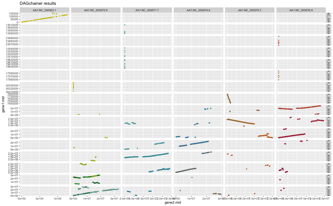
## plot DAGchainer results selected chromosomes
g <- plot_dagchainer(
    dag=ARATHA_ARALYR_crbh.dagchainer.bp,
    select.chr=c(
    "AA1:NC_003070.9", "AA1:NC_003071.7", "AA1:NC_003074.8",
    "AA1:NC_003075.7", "AA1:NC_003076.8",
    "AA2:NW_003302551.1", "AA2:NW_003302554.1",
    "AA2:NW_003302553.1", "AA2:NW_003302552.1",
    "AA2:NW_003302551.1", "AA2:NW_003302550.1",
    "AA2:NW_003302549.1", "AA2:NW_003302548.1"))
g
## change title size
g + ggplot2::theme(title=element_text(size=16))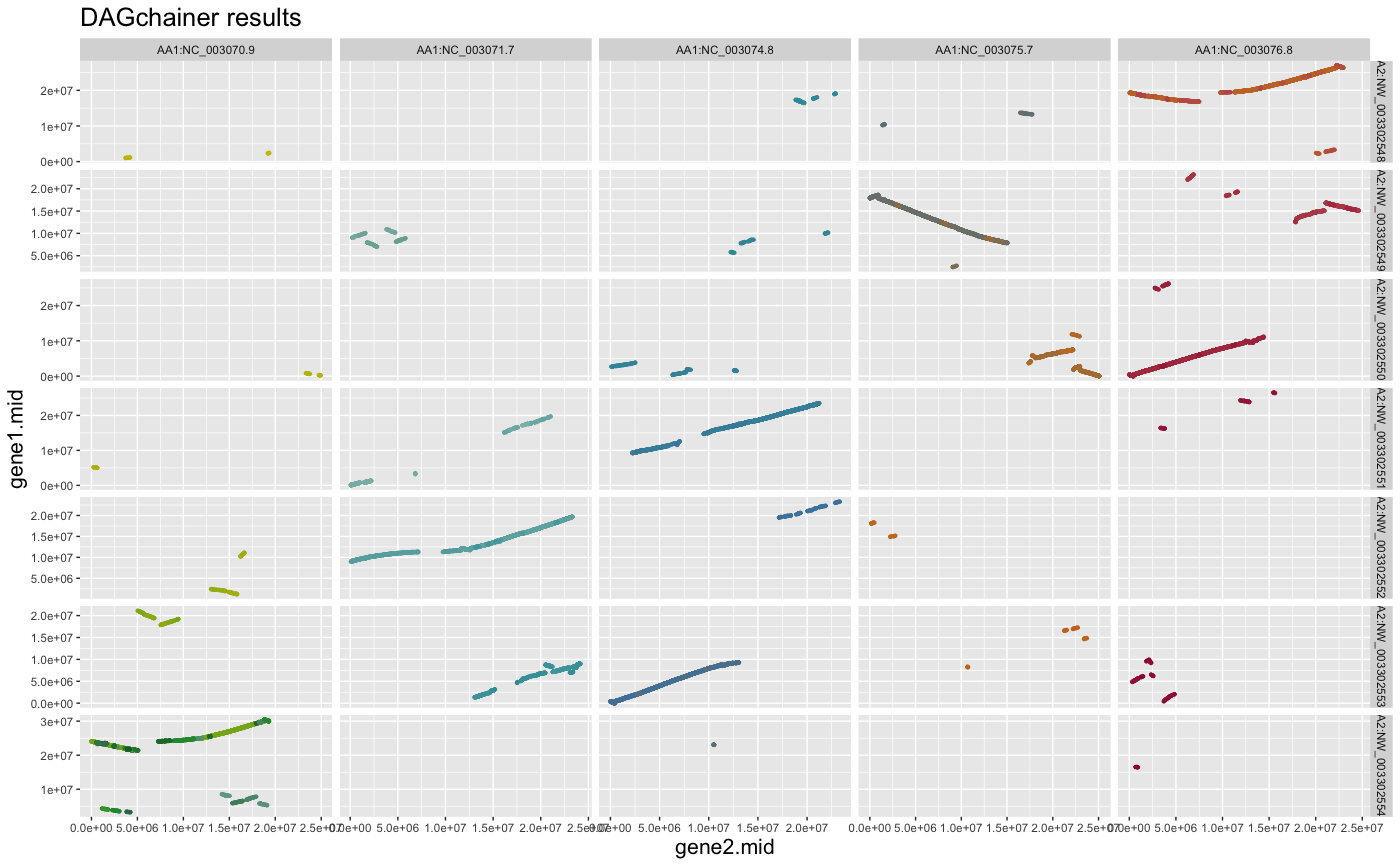
## change axis title size (gene1.mid; gene2.mid)
g + ggplot2::theme(axis.title.x=element_text(size=16),
    axis.title.y=element_text(size=16))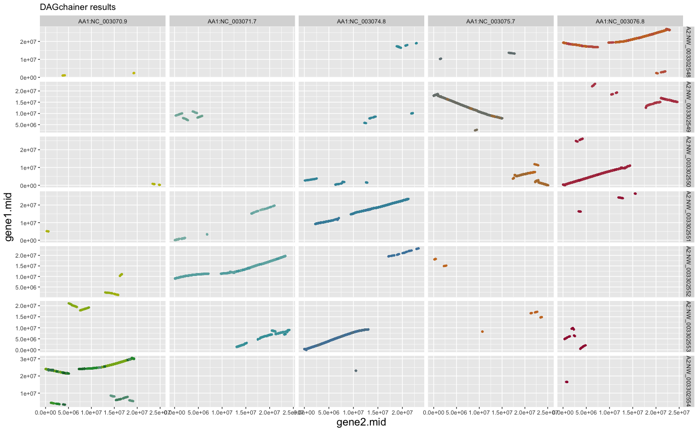
## change grid title size
g + theme(strip.text.x=element_text(size=16), strip.text.y=element_text(size=16))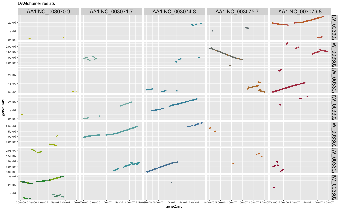
## change grid axis size and angle
g + theme(axis.text.x=element_text(size=12, angle=90))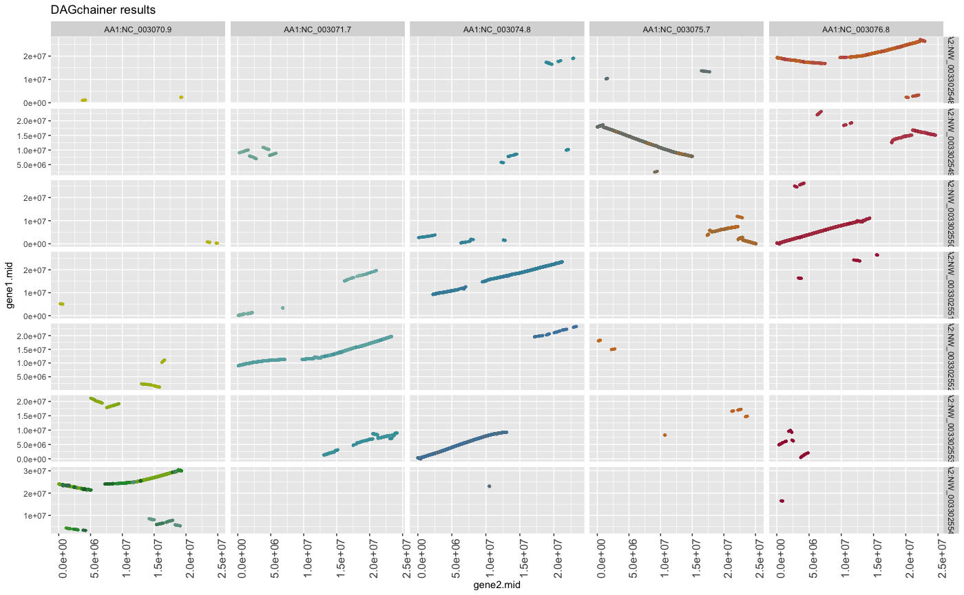
## get help
#?plot_dagchainer
The same analysis can be done just using the selfblast hits of one species.
## example how to run DAGchainer on CRBHit pairs and gene positions
## DAGchainer using gene base pair (gene bp start end)
## ignore tandem duplicates
## Note: change parameter to fit bp option
ARATHA_selfblast_crbh.dagchainer.ignore_tandem.bp <- rbh2dagchainer(
rbhpairs=ARATHA_selfblast_crbh,
gene.position.cds1=ARATHA.cds.longest.genepos,
gene.position.cds2=ARATHA.cds.longest.genepos,
type="bp",
gap_length=10000,
max_dist_allowed=200000,
ignore_tandem=TRUE,
only_tandem=FALSE,
dagchainerpath=vignette.paths[3])
## DAGchainer using gene base pair (gene bp start end)
## use tandem duplicates
## Note: change parameter to fit bp option
ARATHA_selfblast_crbh.dagchainer.tandem.bp <- rbh2dagchainer(
rbhpairs=ARATHA_selfblast_crbh,
gene.position.cds1=ARATHA.cds.longest.genepos,
gene.position.cds2=ARATHA.cds.longest.genepos,
type="bp",
gap_length=10000,
max_dist_allowed=200000,
ignore_tandem=FALSE,
only_tandem=FALSE,
dagchainerpath=vignette.paths[3])
## DAGchainer using gene base pair (gene bp start end)
## use only tandem duplicates
## Note: change parameter to fit bp option
ARATHA_selfblast_crbh.dagchainer.only_tandem.bp <- rbh2dagchainer(
rbhpairs=ARATHA_selfblast_crbh,
gene.position.cds1=ARATHA.cds.longest.genepos,
gene.position.cds2=ARATHA.cds.longest.genepos,
type="bp",
gap_length=10000,
max_dist_allowed=200000,
ignore_tandem=FALSE,
only_tandem=TRUE,
dagchainerpath=vignette.paths[3])
## get help
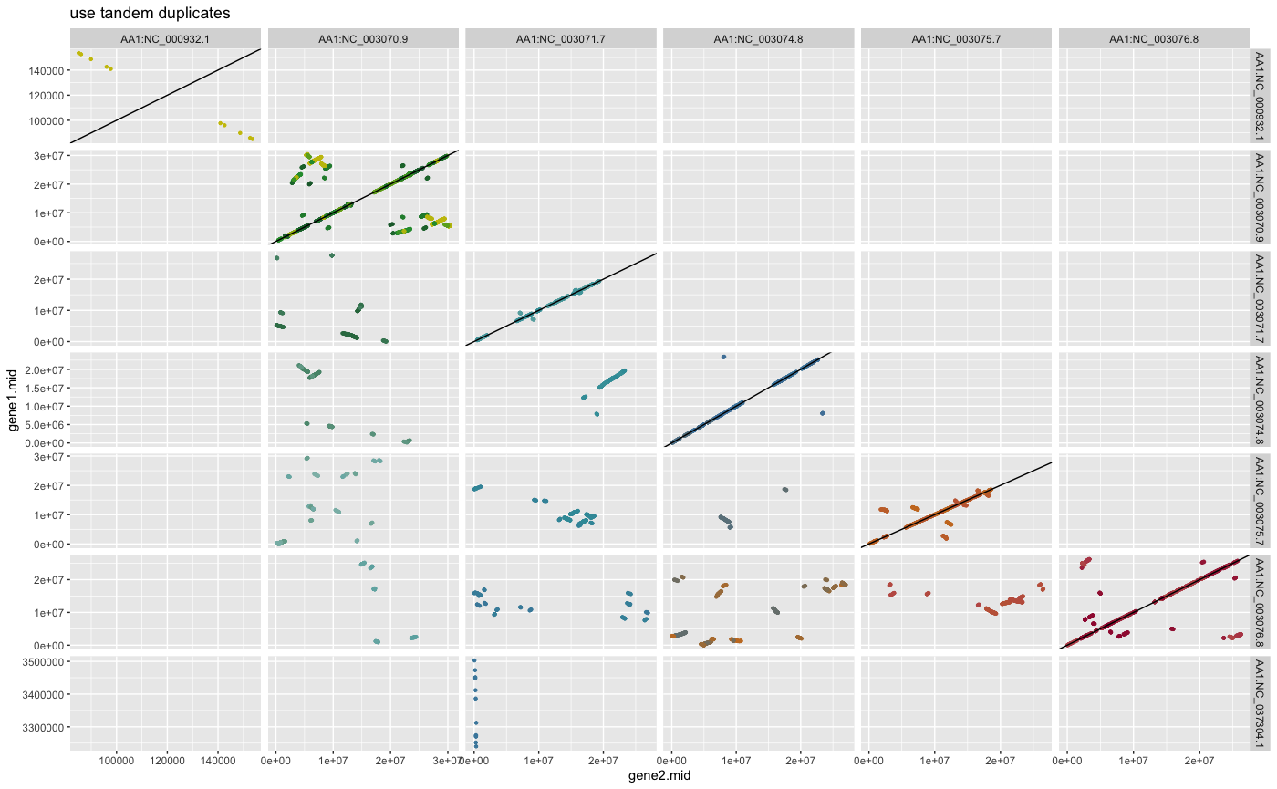
#?rbh2dagchainer## example how to plot pairwise chromosomal syntenic groups for selfblast (DAGchainer results)
## plot DAGchainer results for each chromosome combination
dim(ARATHA_selfblast_crbh.dagchainer.ignore_tandem.bp)
plot_dagchainer(ARATHA_selfblast_crbh.dagchainer.ignore_tandem.bp,
DotPlotTitle="ignore tandem duplicates")
dim(ARATHA_selfblast_crbh.dagchainer.tandem.bp)
plot_dagchainer(ARATHA_selfblast_crbh.dagchainer.tandem.bp,
DotPlotTitle="use tandem duplicates")
dim(ARATHA_selfblast_crbh.dagchainer.only_tandem.bp)
plot_dagchainer(ARATHA_selfblast_crbh.dagchainer.only_tandem.bp,
DotPlotTitle="use only tandem duplicates")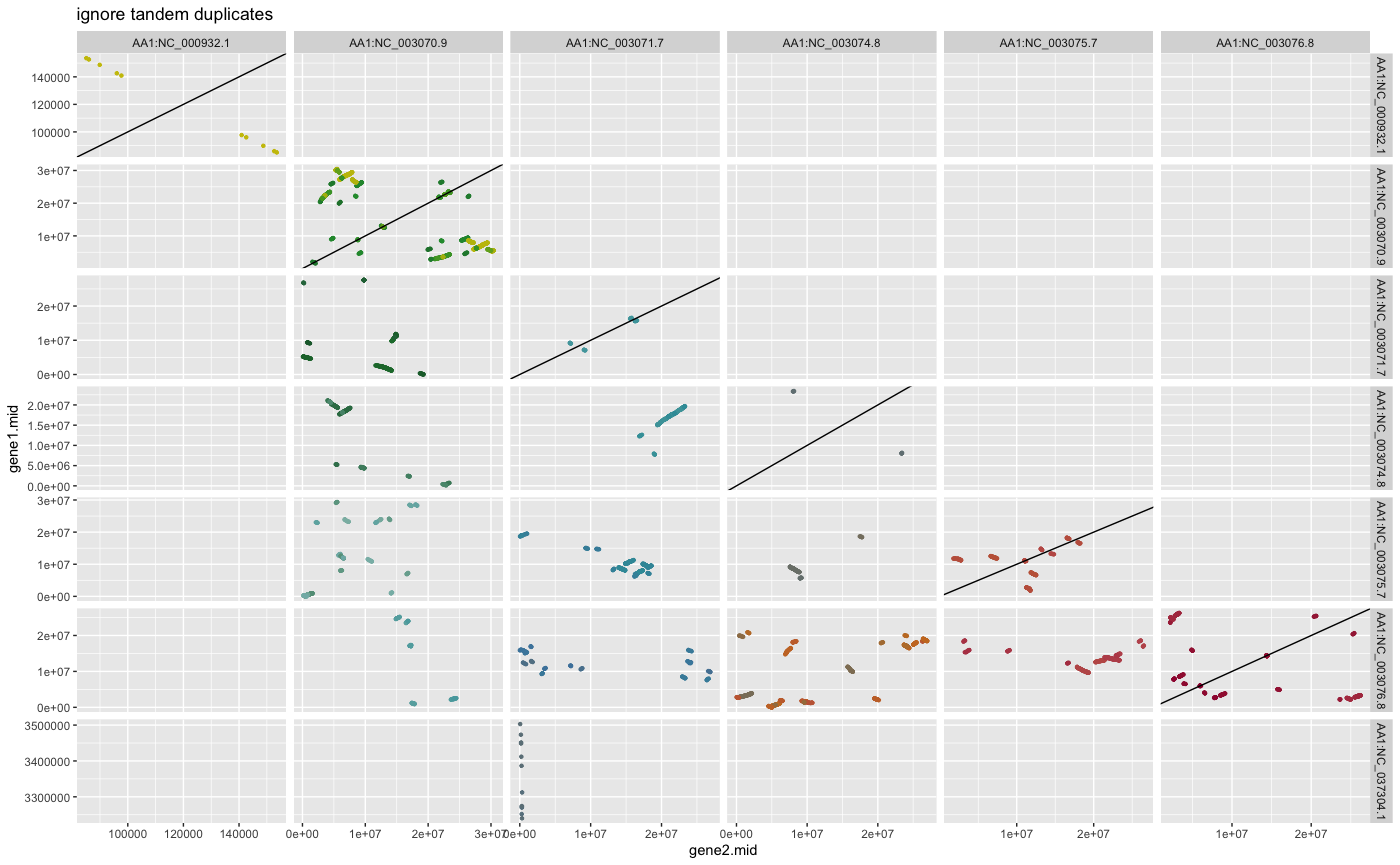

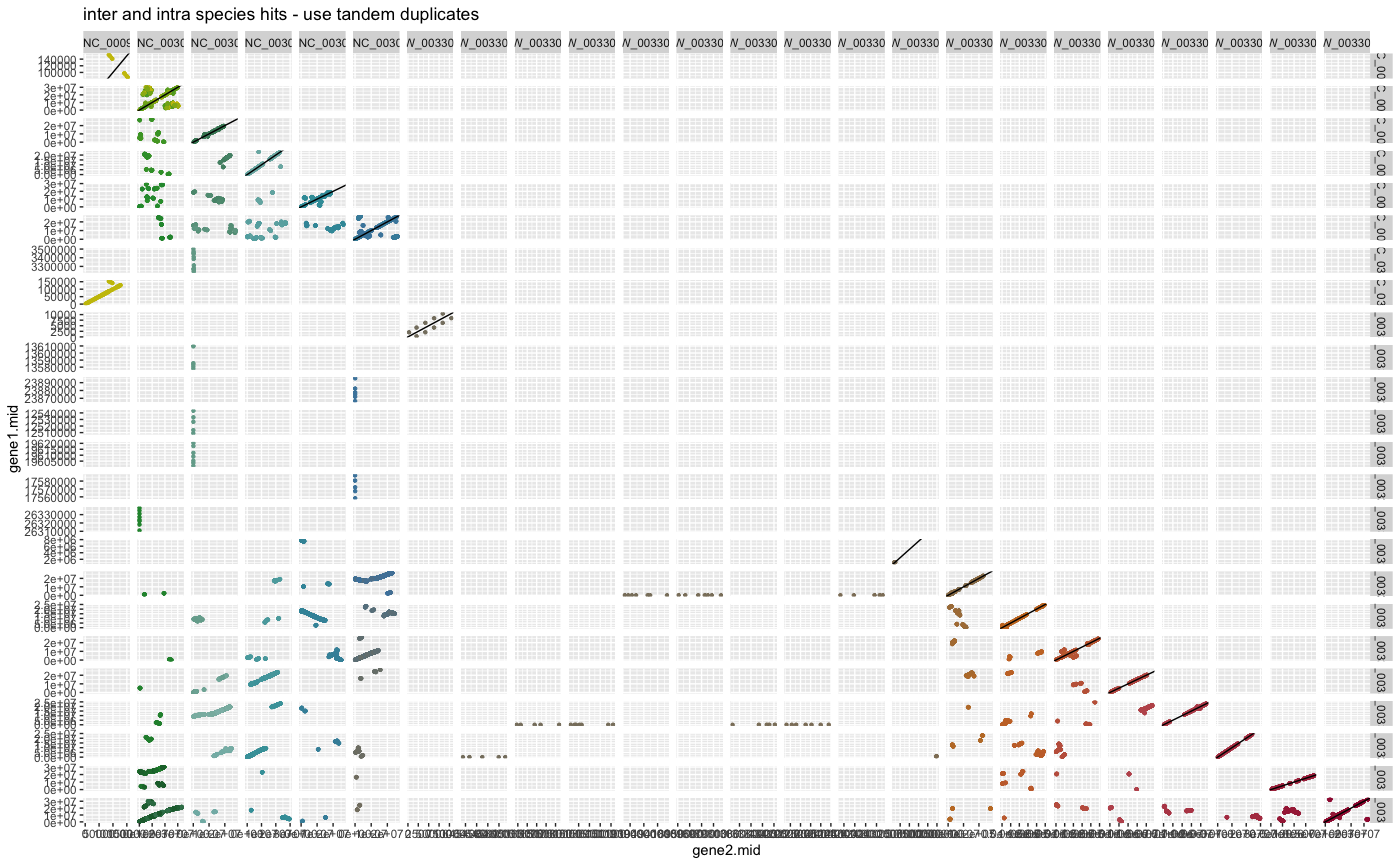
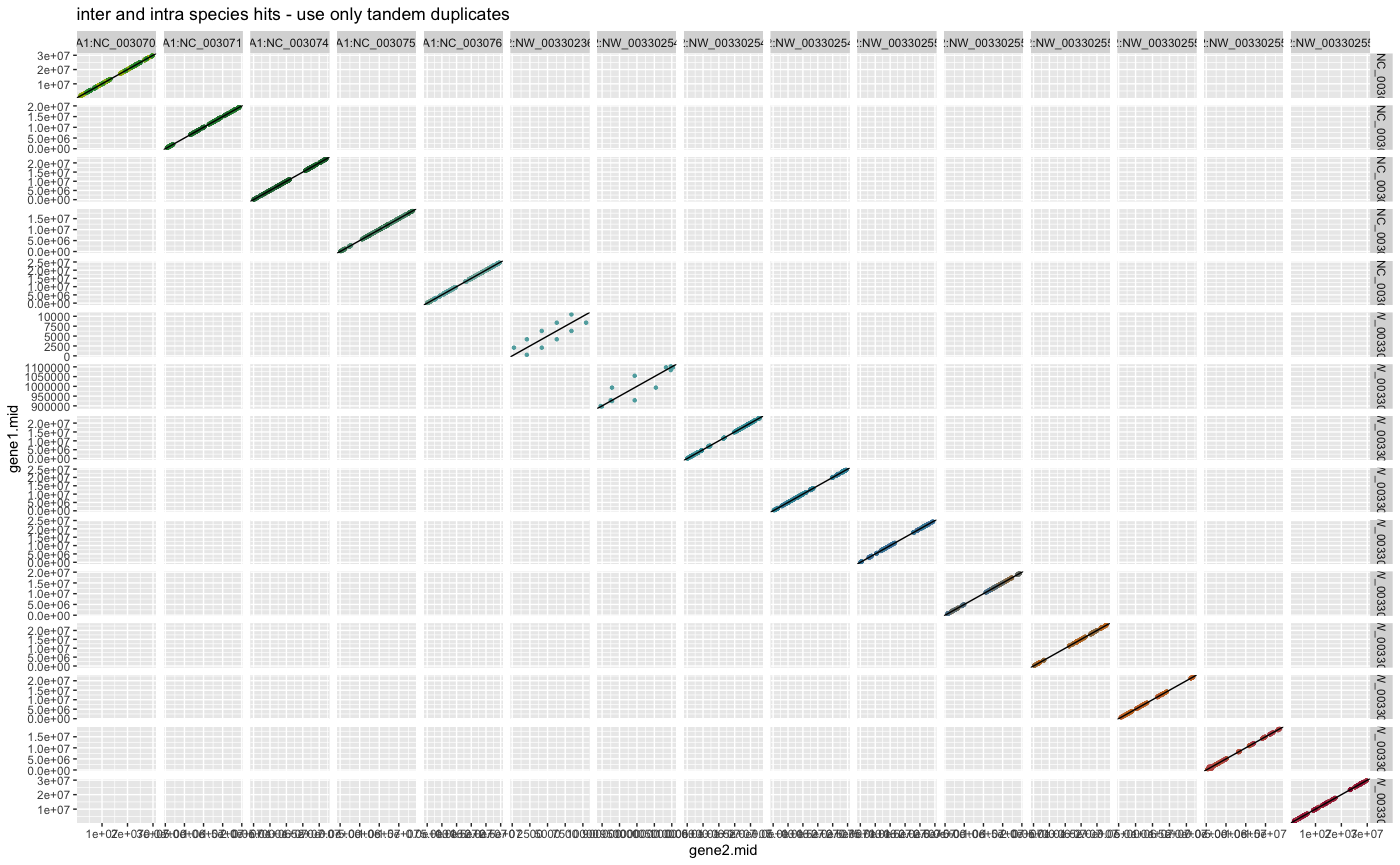
It is even possible to do the same analysis and use the inter and intra species hits.
## example how to run DAGchainer on CRBHit pairs
## and gene positions using inter and intra species hits

## DAGchainer using gene base pair (gene bp start end)
## ignore tandem duplicates
## Note: change parameter to fit bp option
ARATHA_ARALYR_crbh.dagchainer.ignore_tandem.bp <- rbh2dagchainer(
    rbhpairs=ARATHA_ARALYR_crbh,
    selfblast1=ARATHA_selfblast_crbh,
    selfblast2=ARALYR_selfblast_crbh,
    gene.position.cds1=ARATHA.cds.longest.genepos,
    gene.position.cds2=ARALYR.cds.longest.genepos,
    type="bp",
    gap_length=10000,
    max_dist_allowed=200000,
    ignore_tandem=TRUE,
    only_tandem=FALSE,
    dagchainerpath=vignette.paths[3])

## DAGchainer using gene base pair (gene bp start end)
## use tandem duplicates
## Note: change parameter to fit bp option
ARATHA_ARALYR_crbh.dagchainer.tandem.bp <- rbh2dagchainer(
    rbhpairs=ARATHA_ARALYR_crbh,
    selfblast1=ARATHA_selfblast_crbh,
    selfblast2=ARALYR_selfblast_crbh,
    gene.position.cds1=ARATHA.cds.longest.genepos,
    gene.position.cds2=ARALYR.cds.longest.genepos,
    type="bp",
    gap_length=10000,
    max_dist_allowed=200000,
    ignore_tandem=FALSE,
    only_tandem=FALSE,
    dagchainerpath=vignette.paths[3])

## DAGchainer using gene base pair (gene bp start end)
## use only tandem duplicates
## Note: change parameter to fit bp option
ARATHA_ARALYR_crbh.dagchainer.only_tandem.bp <- rbh2dagchainer(
    rbhpairs=ARATHA_ARALYR_crbh,
    selfblast1=ARATHA_selfblast_crbh,
    selfblast2=ARALYR_selfblast_crbh,
    gene.position.cds1=ARATHA.cds.longest.genepos,
    gene.position.cds2=ARALYR.cds.longest.genepos,
    type="bp",
    gap_length=10000,
    max_dist_allowed=200000,
    ignore_tandem=FALSE,
    only_tandem=TRUE,
    dagchainerpath=vignette.paths[3])

## get help
#?rbh2dagchainer
## example how to plot pairwise chromosomal syntenic groups
## for inter and intra species hits (DAGchainer results)
## plot DAGchainer results for each chromosome combination
dim(ARATHA_ARALYR_crbh.dagchainer.ignore_tandem.bp)
plot_dagchainer(ARATHA_ARALYR_crbh.dagchainer.ignore_tandem.bp,
DotPlotTitle="inter and intra species hits - ignore tandem duplicates")
dim(ARATHA_ARALYR_crbh.dagchainer.tandem.bp)
plot_dagchainer(ARATHA_ARALYR_crbh.dagchainer.tandem.bp,
DotPlotTitle="inter and intra species hits - use tandem duplicates")
dim(ARATHA_ARALYR_crbh.dagchainer.only_tandem.bp)
plot_dagchainer(ARATHA_ARALYR_crbh.dagchainer.only_tandem.bp,
DotPlotTitle="inter and intra species hits - use only tandem duplicates")
2. Ka/Ks Calculation
The second part of this vignette describes how to calculate synonymous (Ks) and nonsynonymous substitution rates (Ka) given a set of CRBHit pairs (see Calculate/Filter CRBHit pairs section how to obtain CRBHit pairs).
The rbh2kaks() function is used to obtain pairwise codon
alignments and directly calculate synonymous (Ks) and nonsynonymous (Ka)
substitutions in a parallel fashion. One can choose either to use the
model by Li (1993) or
the model by Yang and
Nielson (2000).
Note:
It is important, that the names of the rbh columns must
match the names of the corresponding cds1 and
cds2 DNAStringSet vectors.
However, since one should directly use the same input
DNAStringSet vector or input url to calculate
the CRBHit pairs with the cds2rbh() or the
cdsfile2rbh() function, this should not be a problem (see
the Get Longest Isoform from NCBI or ENSEMBL
Input section how to obtain the CDS for the next example).
To calculate Ka/Ks values based on the model by Li (1993), do the following:
Note: The following example can take some time and is not calculated by the vignette building process.
## example how to calculate Ka/Ks values with model "Li"

## calculate Ka/Ks using the CRBHit pairs and multiple threads
ARATHA_ARALYR_crbh.kaks.Li <- rbh2kaks(
    rbhpairs=ARATHA_ARALYR_crbh,
    cds1=ARATHA.cds.longest,
    cds2=ARALYR.cds.longest,
    model="Li",
    threads=4)
To calculate Ka/Ks values based on the model by Yang and Nielson (2000), do the following:
Note: The following example can take some time and is not calculated by the vignette building process.
## example how to calculate Ka/Ks values with model "YN"

## calculate Ka/Ks using the CRBHit pairs and multiple threads
ARATHA_ARALYR_crbh.kaks.YN <- rbh2kaks(
    rbhpairs=ARATHA_ARALYR_crbh,
    cds1=ARATHA.cds.longest,
    cds2=ARALYR.cds.longest,
    model="YN",
    threads=4)
3. Ka/Ks Filtering and Visualisation
In some cases the Ka/Ks calculation fails, since e.g. there are no synonymous (Ks) or nonsynonymous substitutions (Ka) between cds1 and cds2 or one wants to get rid of high Ks values due to substitution saturation. One can easily remove these cases before doing further analysis.
A plotting function plot_kaks() is integrated and can be
applied on the Ka/Ks results.
## load example Ka/Ks values (see above commands above how to obtain them)
data("ath_aly_ncbi_kaks", package="CRBHits")

## plot Ka/Ks results as histogram colored by Ka/Ks values
g <- plot_kaks(kaks=ath_aly_ncbi_kaks)
## plot Ka/Ks results as histogram filter for ka.min, ka.max, ks.min, ks.max
g.min_max <- plot_kaks(
    kaks=ath_aly_ncbi_kaks,
    ka.min=0,
    ka.max=1,
    ks.min=0,
    ks.max=1)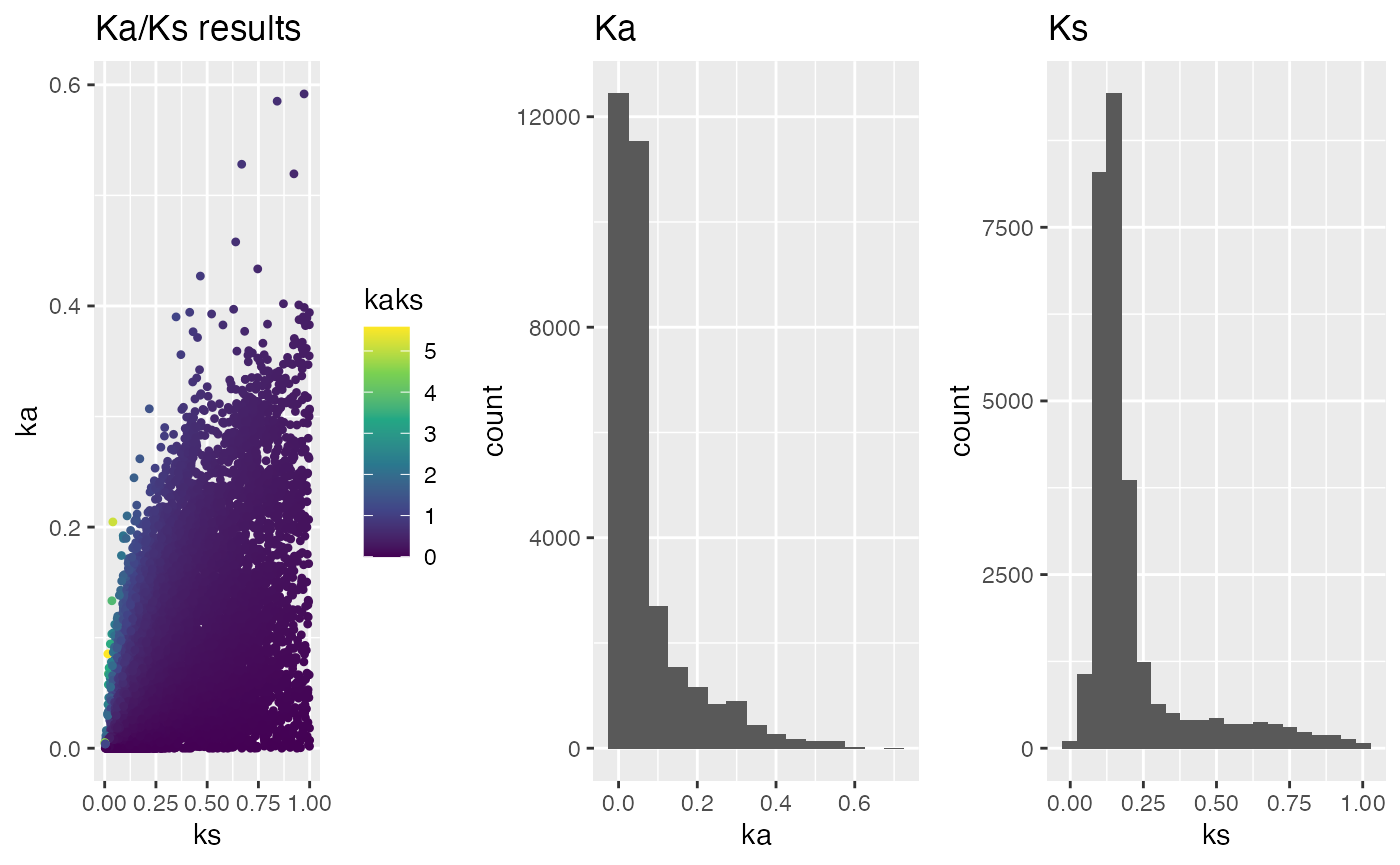
## select subset of chromosomes - needs gene position information
head(ARATHA.cds.longest.genepos)
head(ARALYR.cds.longest.genepos)
g.subset <- plot_kaks(
    kaks=ath_aly_ncbi_kaks,
    gene.position.cds1=ARATHA.cds.longest.genepos,
    gene.position.cds2=ARALYR.cds.longest.genepos,
    select.chr=c(
    "NC_003070.9",
    "NC_003071.7",
    "NW_003302551.1",
    "NW_003302554.1"))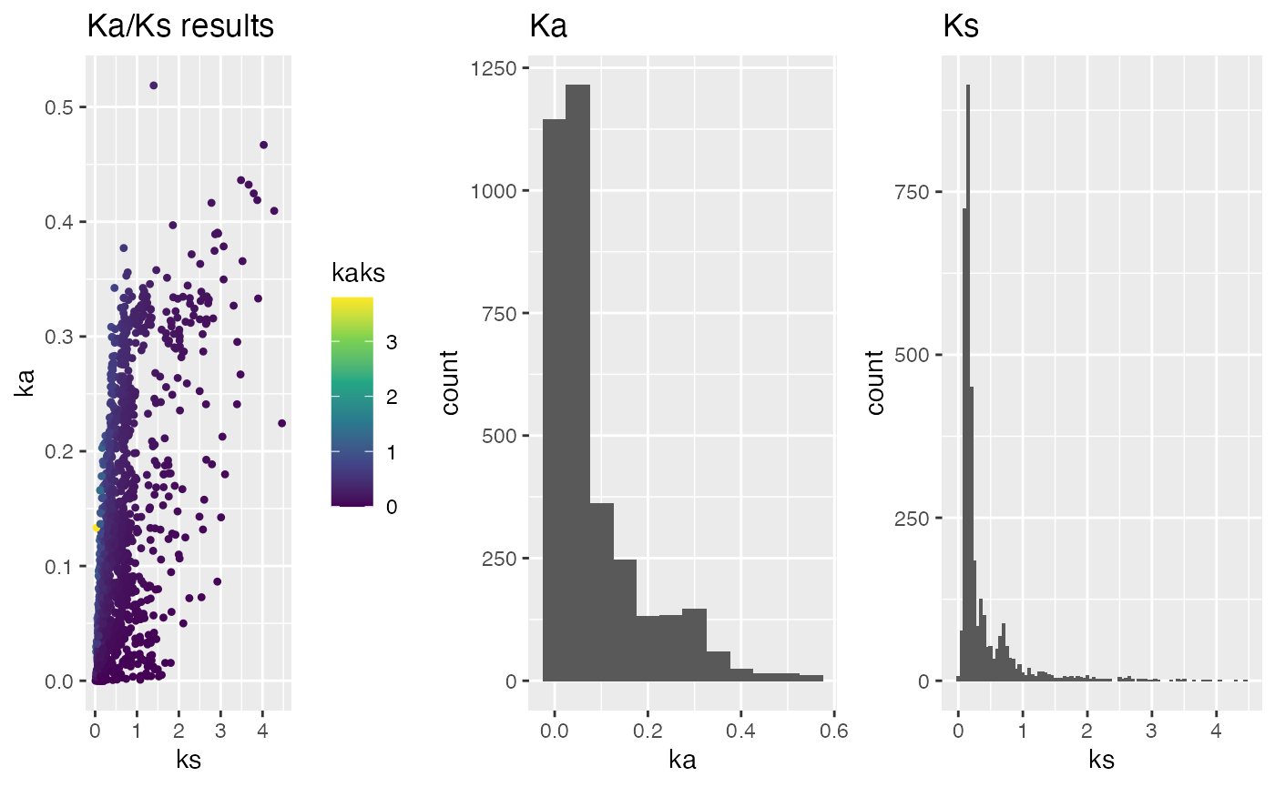
## plot Ka/Ks results and split by chromosome - needs gene position information

g.split <- plot_kaks(
    kaks=ath_aly_ncbi_kaks,
    gene.position.cds1=ARATHA.cds.longest.genepos,
    gene.position.cds2=ARALYR.cds.longest.genepos,
    select.chr=c(
    "NC_003070.9",
    "NC_003071.7",
    "NW_003302551.1",
    "NW_003302554.1"),
    splitByChr=TRUE)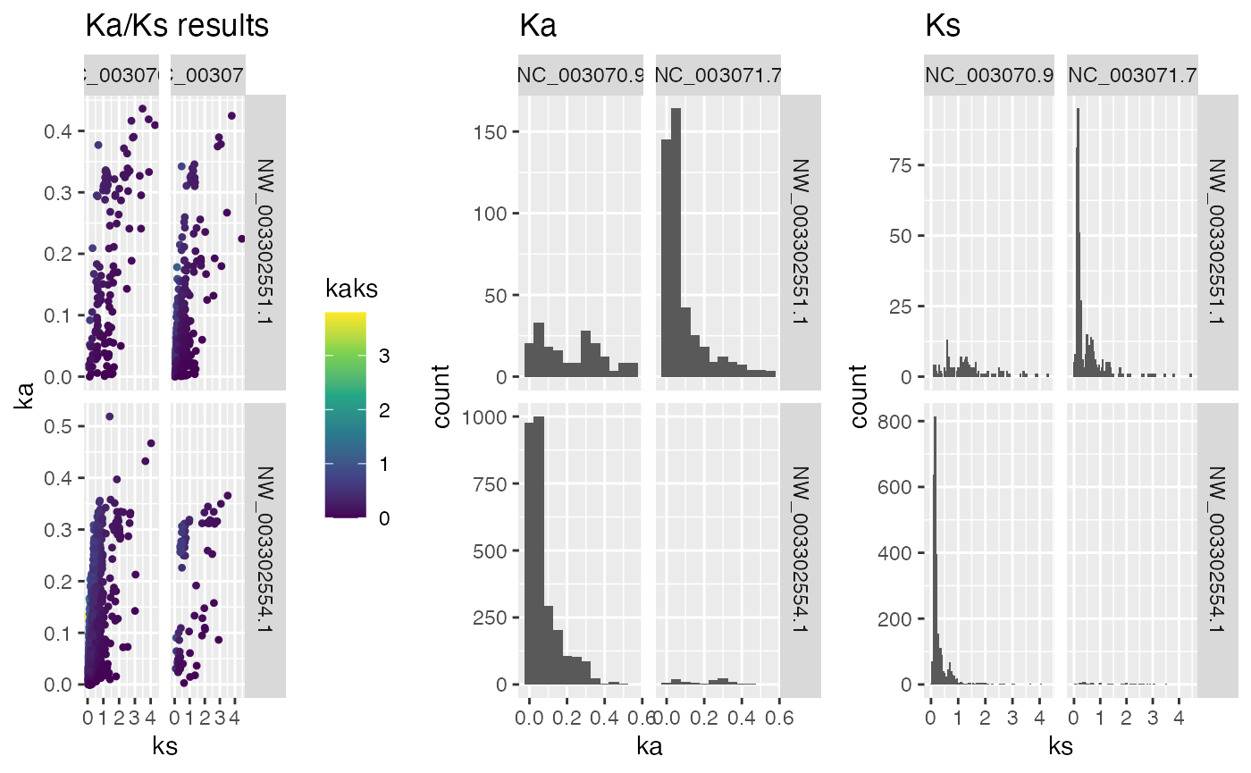
Note: Default data.frame handling with the dplyr package is possible on the original Ka/Ks results as well as on the resulting plot objects.
Apply dplyr::filter() and dplyr::mutate()
function:
## examples how to filter and mutate Ka/Ks results

## filter for Ks values < 2 on original Ka/Ks results
head(ath_aly_ncbi_kaks)
dim(ath_aly_ncbi_kaks)
dim(ath_aly_ncbi_kaks %>% dplyr::filter(ks<2))

## filter for Ks values < 2 on plot object
head(g.split$g.kaks$data)
dim(g.split$g.kaks$data)
dim(g.split$g.kaks$data %>% dplyr::filter(ks<2))

## filter for Ks values < 1 on plot object and plot
g.split$g.kaks$data %>% dplyr::filter(ks<1) %>%
    ggplot2::ggplot() + ggplot2::geom_histogram(binwidth=0.1, aes(x=ks))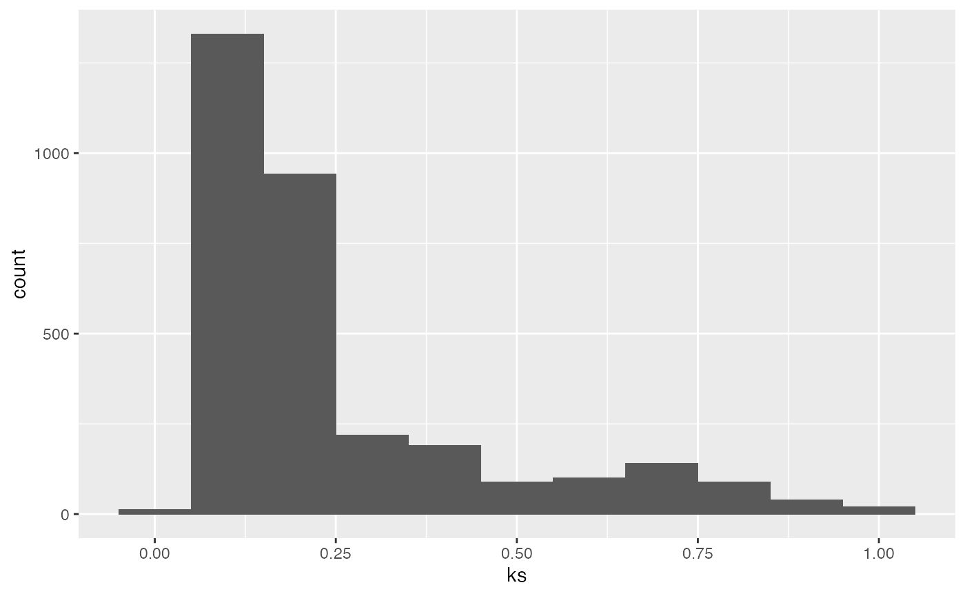
4. Homo sapiens vs. Pan troglodytes example
The second example compares the CDS from Homo sapiens and Pan troglodytes. The input sequences are from the FTP server from Ensembl.
The Ensembl release-101 is used.
## example comparing Homo sapiens and Pan troglodytes

## set URLs for Homo sapiens and Pan troglodytes from Ensembl

## set Ensembl URL
ensembl <- "ftp://ftp.ensembl.org/pub/release-105/fasta/"
## set Homo sapiens CDS URL
HOMSAP.cds.url <- paste0(ensembl,
    "homo_sapiens/cds/Homo_sapiens.GRCh38.cds.all.fa.gz")
## set Pan troglodytes CDS URL
PANTRO.cds.url <- paste0(ensembl,
    "pan_troglodytes/cds/Pan_troglodytes.Pan_tro_3.0.cds.all.fa.gz")

## get Homo sapiens CDS
HOMSAP.cds.file <- tempfile()
download.file(HOMSAP.cds.url, HOMSAP.cds.file, quiet = FALSE)
HOMSAP.cds <- Biostrings::readDNAStringSet(HOMSAP.cds.file)

## get Pan troglodytes CDS
PANTRO.cds.file <- tempfile()
download.file(PANTRO.cds.url, PANTRO.cds.file, quiet = FALSE)
PANTRO.cds <- Biostrings::readDNAStringSet(PANTRO.cds.file)

## get longest isoform
HOMSAP.cds.longest <- isoform2longest(HOMSAP.cds, "ENSEMBL")
PANTRO.cds.longest <- isoform2longest(PANTRO.cds, "ENSEMBL")

## calculate CRBHit pairs for H. sapiens and P. troglodytes using 2 threads

## input from CDS obtained from Ensembl
## longest isoform selection
## query coverage >= 50%
## rost199 filter
HOMSAP_PANTRO_crbh <- cds2rbh(
    cds1=HOMSAP.cds,
    cds2=PANTRO.cds,
    qcov=0.5,
    rost1999=TRUE,
    longest.isoform=TRUE,
    isoform.source="ENSEMBL",
    threads=2,
    plotCurve=TRUE,
    lastpath=vignette.paths[1])
## get gene position for H. sapiens longest isoforms
HOMSAP.cds.longest.genepos <- cds2genepos(
    cds=HOMSAP.cds.longest,
    source="ENSEMBL")
## get gene position for P. troglodytes longest isoforms
PANTRO.cds.longest.genepos <- cds2genepos(
    cds=PANTRO.cds.longest,
    source="ENSEMBL")

## DAGchainer using gene base pair (gene bp start end)
## Note: change parameter to fit bp option
HOMSAP_PANTRO_crbh.dagchainer.bp <- rbh2dagchainer(
    rbhpairs=HOMSAP_PANTRO_crbh,
    gene.position.cds1=HOMSAP.cds.longest.genepos,
    gene.position.cds2=PANTRO.cds.longest.genepos,
    type="bp",
    gap_length=10000,
    max_dist_allowed=200000,
    dagchainerpath=vignette.paths[3])

## plot DAGchainer results for selected chromosome combinations
plot_dagchainer(
    dag=HOMSAP_PANTRO_crbh.dagchainer.bp,
    select.chr=c(
    "AA1:1","AA1:2","AA1:3","AA1:4","AA1:5","AA1:14",
    "AA2:1","AA2:3","AA2:4","AA2:5","AA2:14"))
## get selfblast CRBHit pairs for H. sapiens
HOMSAP_selfblast_crbh <- cds2rbh(
    cds1=HOMSAP.cds,
    cds2=HOMSAP.cds,
    qcov=0.5,
    rost1999=TRUE,
    longest.isoform=TRUE,
    isoform.source="ENSEMBL",
    threads=2,
    plotCurve=FALSE,
    lastpath=vignette.paths[1])
PANTRO_selfblast_crbh <- cds2rbh(
    cds1=PANTRO.cds,
    cds2=PANTRO.cds,
    qcov=0.5,
    rost1999=TRUE,
    longest.isoform=TRUE,
    isoform.source="ENSEMBL",
    threads=2,
    plotCurve=FALSE,
    lastpath=vignette.paths[1])
## example how to run DAGchainer on CRBHit pairs
## and gene positions using inter and intra species hits
## DAGchainer using gene base pair (gene bp start end)
## use tandem duplicates
## Note: change parameter to fit bp option
HOMSAP_PANTRO_crbh.dagchainer.tandem.bp <- rbh2dagchainer(
rbhpairs=HOMSAP_PANTRO_crbh,
selfblast1=HOMSAP_selfblast_crbh,
selfblast2=PANTRO_selfblast_crbh,
gene.position.cds1=HOMSAP.cds.longest.genepos,
gene.position.cds2=PANTRO.cds.longest.genepos,
type="bp",
gap_length=10000,
max_dist_allowed=200000,
ignore_tandem=FALSE,
only_tandem=FALSE,
dagchainerpath=vignette.paths[3])
## plot DAGchainer results for selected chromosome combinations
plot_dagchainer(
dag=HOMSAP_PANTRO_crbh.dagchainer.tandem.bp,
select.chr=c(
"AA1:1","AA1:2","AA1:3","AA1:4","AA1:5","AA1:14",
"AA2:1","AA2:3","AA2:4","AA2:5","AA2:14"))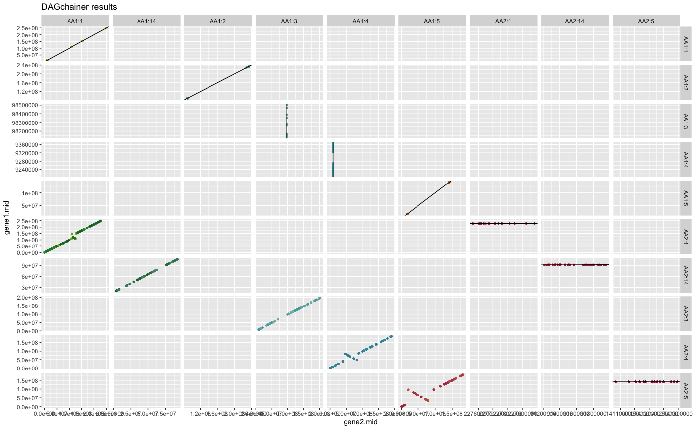
Note: The following example can take some time and is not calculated by the vignette building process.
## example how to calculate Ka/Ks values with model "Li"

## calculate Ka/Ks using the CRBHit pairs and multiple threads
HOMSAP_PANTRO_crbh.kaks.Li <- rbh2kaks(
    rbhpairs=HOMSAP_PANTRO_crbh,
    cds1=HOMSAP.cds.longest,
    cds2=PANTRO.cds.longest,
    model="Li",
    threads=4)
## load example Ka/Ks values (see above commands above how to obtain them)
data("hom_pan_ensembl_kaks", package="CRBHits")
## plot Ka/Ks results as histogram colored by Ka/Ks values
g <- plot_kaks(hom_pan_ensembl_kaks)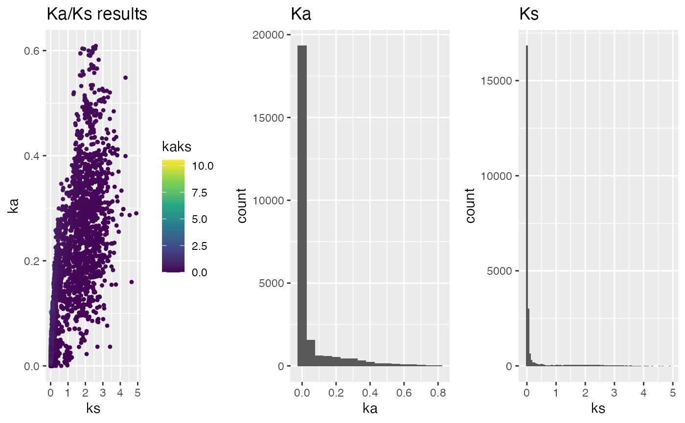
5. References
Aubry S., Kelly S., Kümpers B. M., Smith-Unna R. D., and Hibberd J. M. (2014). Deep evolutionary comparison of gene expression identifies parallel recruitment of trans-factors in two independent origins of C4 photosynthesis. PLoS Genetics, 10(6). https://doi.org/10.1371/journal.pgen.1004365
Charif D., and Lobry J. R. (2007). SeqinR 1.0-2: a contributed package to the R project for statistical computing devoted to biological sequences retrieval and analysis. In Structural approaches to sequence evolution (pp. 207-232). Springer, Berlin, Heidelberg. https://link.springer.com/chapter/10.1007/978-3-540-35306-5_10
Duong T., and Wand M. (2015). feature: Local Inferential Feature Significance for Multivariate Kernel Density Estimation. R package version 1.2.13. https://cran.r-project.org/web/packages/feature/
Haas B. J., Delcher A. L., Wortman J. R., and Salzberg S. L. (2004). DAGchainer: a tool for mining segmental genome duplications and synteny. Bioinformatics, 20(18), 3643-3646. https://doi.org/10.1093/bioinformatics/bth397
Haug-Baltzell A., Stephens S. A., Davey S., Scheidegger C. E., Lyons E. (2017). SynMap2 and SynMap3D: web-based wholge-genome synteny browsers. Bioinformatics, 33(14), 2197-2198. https://academic.oup.com/bioinformatics/article/33/14/2197/3072872
Kiełbasa S. M., Wan R., Sato K., Horton P., and Frith M. C. (2011). Adaptive seeds tame genomic sequence comparison. Genome Research, 21(3), 487-493. https://doi.org/10.1101/gr.113985.110
Kimura M. (1977). Preponderance of synonymous changes as evidence for the neutral theory of molecular evolution. Nature, 267, 275-276.
Li W. H. (1993). Unbiased estimation of the rates of synonymous and nonsynonymous substitution. Journal of Molecular Evolution, 36(1), 96-99. https://doi.org/10.1007/bf02407308
Microsoft, and Weston S. (2020). foreach: Provides Foreach Looping Construct. R package version, 1.5.1. foreach
Mugal C. F., Wolf J. B. W., Kaj I. (2014). Why Time Matters: Codon Evolution and the Temproal Dynamics of dN/dS. Molecular Biology and Evolution, 31(1), 212-231.
Ooms J. (2019). curl: A Modern and Flexible Web Client for R. R package version, 4.3. curl
Pagès H., Aboyoun P., Gentleman R., and DebRoy S. (2017). Biostrings: Efficient manipulation of biological strings. R package version, 2.56.0. Biostrings
Revolution Analytics, and Weston S. (2020). doMC: Foreach Parallel Adaptor for ‘parallel’. R package version, 1.3.7. doMC
Rost B. (1999). Twilight zone of protein sequence alignments. Protein Engineering, 12(2), 85-94. https://doi.org/10.1093/protein/12.2.85
Scott C. (2017). shmlast: an improved implementation of conditional reciprocal best hits with LAST and Python. Journal of Open Source Software, 2(9), 142. https://joss.theoj.org/papers/10.21105/joss.00142
Scrucca L., Fop M., Murphy T. B., and Raftery A. E. (2016) mclust 5: clustering, classification and density estimation using Gaussian finite mixture models. The R Journal, 8(1), 289-317. https://www.ncbi.nlm.nih.gov/pmc/articles/PMC5096736/
Wickham H. (2011). testthat: Get Started with Testing. The R Journal, 3(1), 5. testthat
Wickham H. (2019). stringr: Simple, Consistent Wrappers for Common String Operations. R package version, 1.4.0. stringr
Wickham H. (2020). tidyr: Tidy Messy Data. R package version, 1.1.2. tidyr
Wickham H., Hester J., and Chang W. (2020). devtools: Tools to make Developing R Packages Easier. R package version, (2.3.2). devtools
Wickham H., François R., Henry L., and Müller K. (2020). dplyr: A Grammar of Data Manipulation. R package version, 1.0.2. dplyr
Yang Z., and Nielsen R. (2000). Estimating synonymous and nonsynonymous substitution rates under realistic evolutionary models. Molecular Biology and Evolution, 17(1), 32-43. https://doi.org/10.1093/oxfordjournals.molbev.a026236